AirROI Dynamic Pricing Engine Overview


The AirROI dynamic pricing engine is a third-generation model trained on more than 15 years of transaction history across 20 million properties and refined against billions of new booking signals every day. It prices any short-term rental night anywhere, and every recommendation comes with a dollar-level receipt attributing the result to the property foundation, recurring seasonality, and live market demand.
We'd love to show you how it's built. The receipt below is one night of output: a Saturday in Miami Beach during the 2026 World Cup.
ADJUSTMENT EXPLANATIONS
The big idea
The engine builds a nightly price from three factors, each estimated from the evidence that speaks to it.
- Property foundation. What this specific property is worth on an ordinary night, with seasonal effects removed. Determined by location, size, capacity, and attributes against the transacted prices of comparable properties nearby.
- Recurring seasonality. The predictable annual rhythm of the property's neighborhood: high and low seasons, weekday contrasts, public holidays, school breaks. Learned from years of confirmed bookings.
- Market demand. Booking pressure for a specific night, above or below what the season predicts. Festivals, championship weekends, holidays with unusual travel, and soft periods live here. Estimated from current booking signals.
Confirmed bookings establish what a property is worth and how its neighborhood's year is shaped. Live booking signals measure what is happening to a specific night. Host rules are applied last and always take precedence.
Host rules apply after the model: minimum and maximum prices, weekday adjustments, last-minute discounts, occupancy pacing, and fixed overrides. Rules are applied last and always take precedence.
The output is a sequential price attribution: a signed dollar contribution for each stage that sums exactly to the served price, as on the receipt at the top of this document.
Getting technical. The property foundation is a structural booked-price center estimated by gradient-boosted tree models over location and attribute features, with the seasonal component projected out before fitting and reinstated at the level. A new listing with no history receives its foundation from comparable properties and its neighborhood, and the estimate shifts toward its own bookings as they accumulate.
Extracting seasonality patterns
The recurring calendar is the backbone of every recommendation. It is estimated from confirmed bookings, within properties, with three methods.
Estimating within properties
The seasonal model is a panel econometric regression on log booked price with listing-year fixed effects: a separate intercept for each property in each year.
The intercepts absorb what each property costs; the seasonal term absorbs when it costs more. Each property is compared with itself across the year, so the fitted shape reflects how prices move through the calendar rather than which properties happened to book in which month. Asking prices are excluded from the fit: an asking price is a host's decision, a booked price is a market outcome, and listings that never book still post prices that carry their owners' errors.
Spectral decomposition of the annual shape
The seasonal term is represented by Fourier spectral decomposition: a sum of smooth periodic waves at the annual frequency and its overtones. One wave can draw a single peak. Several waves together can draw anything a year does, including two peaks, long shoulders, and sharp holiday weeks, with continuous transitions between seasons rather than monthly steps.
Kyoto is the test case. It has two premium seasons, spring and autumn, and a single-wave model is forced to choose one.
A smooth annual curve is a sum of periodic waves. One wave can only draw a single peak. Add waves and Kyoto's spring and autumn peaks appear — nobody told the model Kyoto has two seasons.
The same basis carries weekday contrasts, country-specific public holidays, and school-break timing, so the recurring calendar is one coherent multi-harmonic seasonal decomposition rather than a stack of separate adjustments.
Hierarchical shrinkage across geographies
A single neighborhood may record only a few hundred bookings a year, too few to estimate its own annual curve reliably. A city-wide curve is reliable but wrong for many of its neighborhoods. The engine resolves this with a mixed-effects hierarchical framework fit across multiple geographic resolutions at once. Each local curve is estimated with shrinkage toward the curve of the region that contains it, a form of hierarchical partial pooling in the James-Stein family:
With little local evidence (n small) the served curve leans on the parent region; as evidence accumulates the local shape takes over. The pooling strength is a function of the evidence, not a per-market setting.
A neighborhood with a handful of bookings cannot draw a reliable annual curve alone. The engine shrinks its noisy local estimate toward the surrounding region's curve — and lets go as local evidence accumulates.
This is transfer learning across geographies. Mediterranean summer markets share a broad seasonal structure while keeping their own amplitudes: Santorini, Ibiza Town, and Albufeira all peak in summer at 1.61×, 1.92×, and 2.08× their winter prices respectively. The hierarchy learned the differences from each market's own bookings.
Getting technical. The recurring model minimizes a weighted squared error in log booked price with the listing-year intercepts absorbed through sufficient statistics and a penalty that pulls each geography's coefficients toward its parent's. Observations are recency-weighted with a multi-year half-life; extreme booked rates are bounded with robust M-estimation (winsorization) at the cell-day level. The fitted curve is normalized to a mean of one over the forecast year, so shape and level remain separate objects.
Every coefficient is hyper-local and refreshed against current transaction data. None is a national average or a hand-built seasonal template.
Seasonality in 12 markets
The grid below shows the engine's recurring seasonal factor for a standardized two-bedroom in twelve markets, on one shared scale. The curves are the model's own output for the September 2026 release; no market received a manual override.
The engine's recurring seasonal factor for a standardized two-bedroom in each market, by week of the year, on one shared scale. 1.0 is the property's own annual average; the ratio in each corner is the recommended peak-month to low-month price ratio.
Observations:
- Miami Beach peaks in winter at 1.41× its late-summer low. A beach-means-summer template prices it backwards.
- Kyoto has two peaks, April and November, at 1.46×. A single-peak model cannot represent it.
- Ski markets differ in depth. Park City runs 2.34× from ski season to autumn shoulder, Whistler 2.05×, Breckenridge 1.93×, Niseko 1.43×. The hierarchy preserved the differences rather than averaging them.
- Mediterranean summers share a shape, not an amplitude: Albufeira 2.08×, Ibiza Town 1.92×, Santorini 1.61×, Palma 1.54×.
- Scottsdale and Myrtle Beach are both US leisure markets with opposite years: desert winter at 1.64× and summer beach at 2.10×.
Hyper-local neighborhood pricing
Neighborhoods within one city can run on different calendars, and a city-level model prices both of them wrong. Two examples follow, at two distances.
Daytona Beach: oceanfront and the Speedway corridor, 7.7 km apart
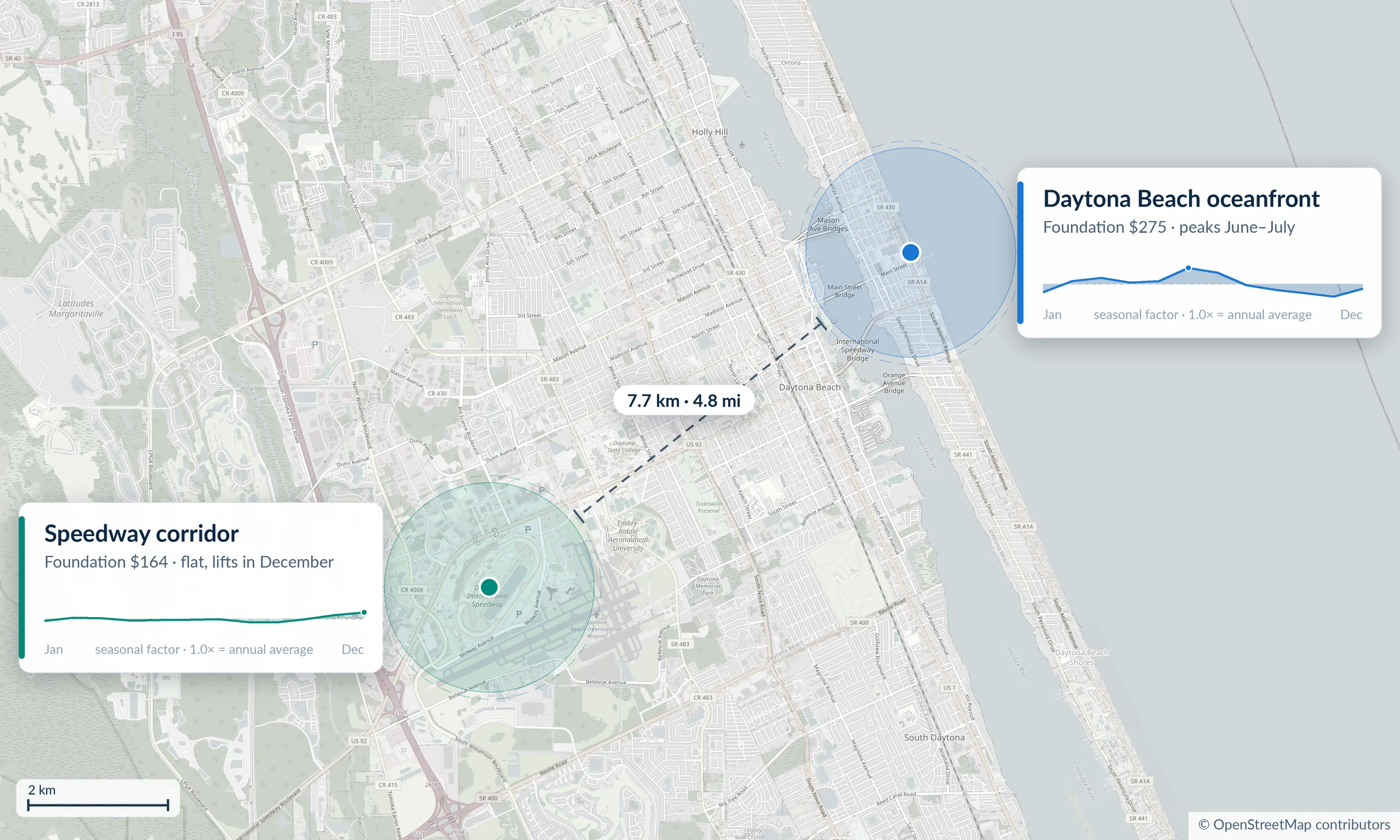
A two-bedroom on the oceanfront has a foundation price of $275 and a classic Atlantic beach calendar: the June–July peak runs about 18% above the property's annual average, November about 13% below. The same two-bedroom 7.7 km inland, in the corridor around the Speedway, the airport, and the interstate, has a foundation price of $164 and an almost flat calendar whose only lift is December. In July and again in November the two locations move in opposite directions.
Weekly recommendations for the same two-bedroom on the Daytona Beach oceanfront and in the Speedway corridor inland, each indexed to its own annual average. The beach has a summer season; the inland corridor is flat with a December lift.
The engine resolved both the level and the shape of the calendar at neighborhood scale. A single Daytona curve would give the inland property a summer premium it cannot earn and take away the beach's.
Austin: Downtown and Lake Travis, 22 km apart
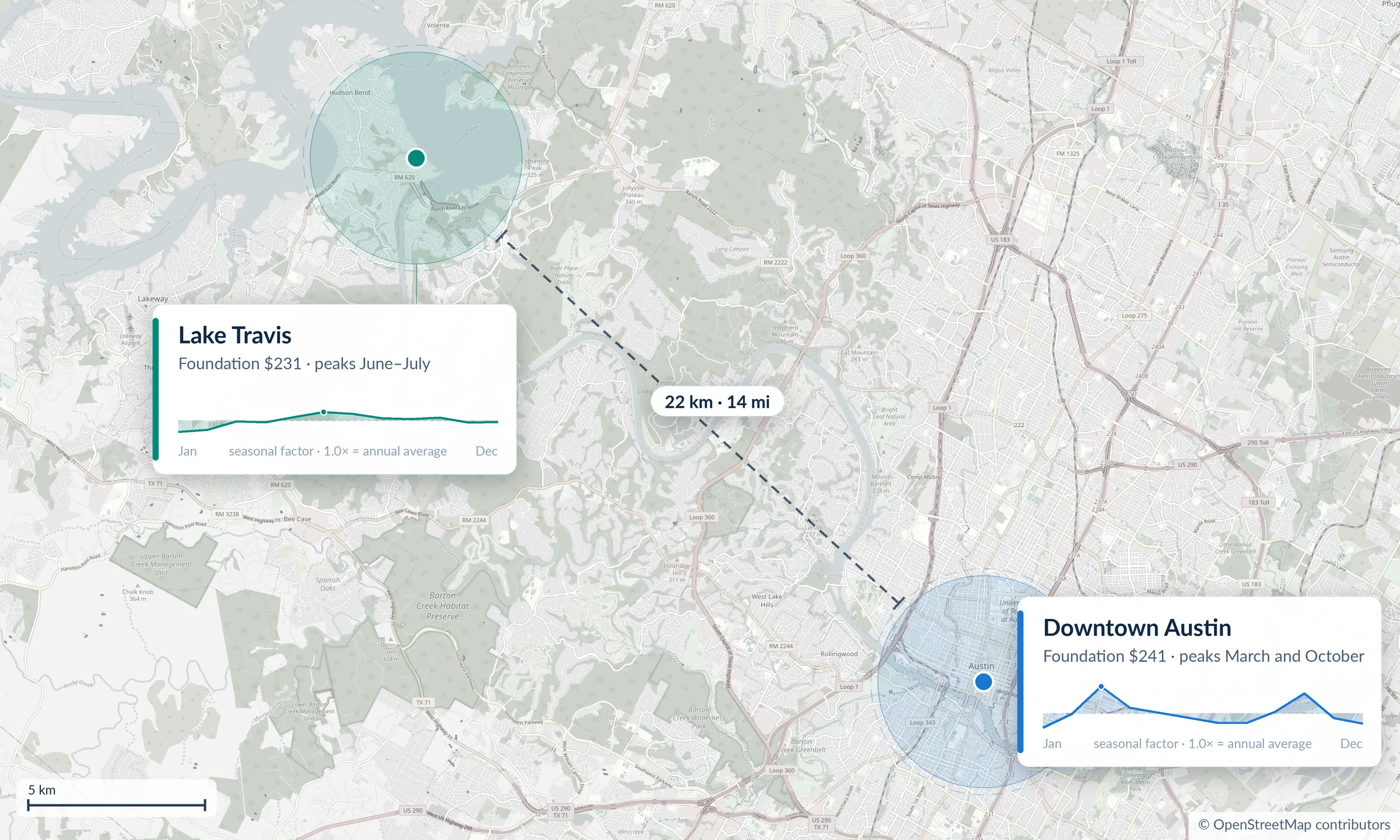
Here the foundation prices are almost the same, $241 and $231, and the calendars are opposite. Downtown peaks in March on SXSW and in October on ACL Festival and the United States Grand Prix, and softens in the July heat. Lake Travis peaks in June and July and does not register SXSW.
Weekly recommendations for the same two-bedroom in Downtown Austin and on Lake Travis, each indexed to its own annual average. Same city, nearly the same foundation price, opposite calendars.
A city-wide seasonal curve for Austin would assign the lake house a March premium nobody will pay and remove the July premium it has earned. Every recurring and demand coefficient in the engine is resolved at neighborhood scale, with the hierarchy of the seasonality section supplying regional support where local evidence is thin.
Booking probability explained
A short-term rental night is sold once or not at all. Demand for it is therefore not a quantity but a probability: the chance that the night books at a given price. Call that probability q(p). It falls as the price rises, and the shape of that fall is the night's price elasticity.
Expected revenue for the night is the price multiplied by the probability of earning it:
A low price books almost every time and earns little. A high price earns a lot on the rare occasion it books. The best price is between them, where the expected revenue curve peaks. At that point the elasticity of booking probability with respect to price is exactly one: a 1% price increase loses 1% of booking probability, and any further increase loses more probability than it gains in price.
For a single night, demand is a probability: the chance the night books at a given price. Expected revenue is price times that probability, and it peaks well before the probability reaches zero.
Two things move the curve. A high-demand night shifts it to the right: at every price, more guests are willing to book, so the optimum moves up while the booking probability at the optimum barely changes. That shift is exactly what the market demand factor measures. A more price-sensitive market steepens the curve and pulls the optimum down; sensitivity differs by neighborhood and by season, and the engine estimates it rather than assuming it.
Getting technical. The engine does not assume a parametric form for q(p). Booking probability is calibrated against an empirical, non-parametric distribution of comparable transacted prices at similar lead times, resolved per neighborhood. Price is also a quality signal, so the empirical curve is not required to be monotone at the low end: a listing priced far below its comparables can book less often, not more.
Lead time changes the answer
The probability that a night books is not fixed. It depends on how far away the night is, because bookings for a given date accumulate along a curve as the date approaches. Write B(t) for the share of comparable nights already booked t days before arrival and F for the share that will be booked by arrival. A night that is still open at lead time t books before arrival with probability:
If comparable nights finish at 88% occupancy and 12% are booked 240 days out, an open night at that lead time has an 86% chance of booking. At 14 days out, with 76% already booked, the same open night has a 50% chance. The market outlook has not changed; the probability for this night has, and the price that maximizes its expected revenue has moved with it.
Grey curves are how comparable past dates filled as they approached. The blue curve is a night 120 days from check-in, observed so far. The engine reads two things from it: how far ahead of the reference it is (pacing) and how fast it has moved lately (pickup).
An open night also has option value. Turning down a low price a year out keeps the chance of a better booking later; a week out, that chance is nearly gone. The value of an open night at each lead time can be written as a recursion: the best price today balances what booking now earns against what the night is still worth if it stays open one more day.
The consequence is the pricing behavior hosts observe in practice: a premium far out, when option value is high and early bookers are the least price-sensitive, and a measured decline for nights that remain unsold as arrival approaches. When a night books faster than its expected curve, the same logic runs in reverse and the recommendation rises.
Getting technical. The engine models the booking curve with methods from survival analysis. Each night has a daily booking hazard h(t), the probability it books on a given day given that it is still open, and the booked share B(t) is one minus the survival function S(t). The expected hazard is specific to the market, property type, season, and lead time. Lead-time-conditioned demand estimation compares observed booking pace and velocity against that expectation, so 60% booked reads as strong evidence nine months out and as ordinary two weeks out. The recursion above is the principle; in production the lead-time-conditioned hazard and the price response are estimated directly from comparable transactions rather than solved night by night.
Event and demand response
Recurring seasonality cannot explain Oktoberfest. The season says ordinary autumn; the bookings say otherwise. Market demand is the factor that measures the shift in the booking-probability curve for a specific night, in both directions.
Signals
The demand estimators ingest a wide array of hyper-local, continuously refreshed booking signals: booking pace against the expected curve, booking velocity, booked-price behavior, statistical support, persistence across successive observation windows, and more. The signals are geographically granular at the same multi-resolution scale as the seasonal model, and they update as new bookings appear. No single signal decides that demand is exceptional.
Market demand does not depend on an event being named. Known holidays and scheduled events have their own line on the receipt; the demand factor measures what the bookings show beyond that line, so an unnamed festival, a conference, or a surge with no calendar entry is priced from the surge itself. The mega-event section below shows eight such responses, none of which relied on an event-specific model.
Evidence-gated ensemble
Several specialized demand estimators operate inside the engine. Each is evidence-gated: it is admitted into the final estimate only when the evidence clears its gate, and the estimators capable of recommending the largest increases require the most agreement across signals.
Several specialized demand estimators exist, but each is admitted only when the evidence clears its gate. The strongest responses require the most agreement.
This design answers the question hosts ask first: will the engine price a property out of its own bookings? The largest responses are reserved for nights where pace, velocity, price behavior, and persistence all point the same way. Ambiguous evidence produces measured moves. On a soft night the demand factor lowers the recommendation below the seasonal price rather than holding a number the market will not pay.
Getting technical. The upper-quantile estimators are monotonic gradient-boosted quantile regressions: they target a conditional upper quantile of the supported price response and carry explicit monotonic constraints on declared features, so more evidence cannot produce a smaller response through that path. Estimator outputs are combined in log-price space.
Pricing above the observed market
If the observed booked median for Oktoberfest nights is $620, the engine may still recommend $780. The booked median is a sample of what hosts chose to charge and guests accepted, not the ceiling of what guests would have accepted. Booked prices are used for calibration and plausibility bounds; they are not treated as a counterfactual. When pace, velocity, and price behavior indicate that the booking-probability curve has shifted right, recommending above the observed median is the correct inference.
Demand response at 8 mega-events
The grid below shows daily recommendations in the weeks around eight major events, with the seasonal-only price alongside the final recommendation. The ratio in each tile compares event nights to matching-weekday nights outside the event window.
Daily recommendations for a standardized two-bedroom in the weeks around each event. The teal line is what recurring seasonality alone would price; the blue line adds market demand. The shaded nights are the event; the ratio in each corner compares event nights to matching-weekday nights outside the window.
Observations:
- Oktoberfest, Munich: 2.68×. A sixteen-night response above a moderate autumn baseline, with the demand factor near 2.0× for most of the run.
- Formula 1 in three cities. Austin 2.28×, Mexico City 1.83×, Abu Dhabi 2.55×. Same event category, three different local contexts. Abu Dhabi's flat local season makes its surge fully incremental; Mexico City's race overlaps Día de Muertos, which the recurring calendar already partly prices.
- Sydney New Year's Eve: 2.38×. A three-night peak rising out of an already elevated Australian summer.
- Coachella weekend one, Indio: 2.46×. Festival demand added on top of the desert spring season.
- Mardi Gras, New Orleans: 2.22× across five nights.
- Carnival, Rio de Janeiro: 1.60×. The smallest ratio in the grid, because Rio's high summer is already carried by recurring seasonality. The demand factor adds only the increment the calendar does not explain. An engine that did not separate the two factors would either double-count the summer or under-price the event.
How an event night fills
The booking curves of the Lead time section, observed in one market. Twelve Scottsdale stay dates, tracked as they approached: ordinary nights travel together in a band, while the Phoenix Open, spring training, and Barrett-Jackson auction week leave the band six months out and never return.
For twelve Scottsdale stay dates, the share of two-bedroom homes already booked as each date approached — one line per date, observed month by month. Read from left to right as check-in nears.
Anecdotal results
Hosts who move to the engine earn 15 to 45% more: the low end of that range against competing dynamic pricing products, the high end against manual or flat pricing. Against tools that charge per listing per month or take a share of revenue, the engine costs 50 to 90% less, and there is no lower tier of the model: a single-property host and a thousand-unit operator run the same code path and receive the same receipts.
Limitations
- No model is right every night. Pricing is probabilistic. Weather, regulation, airline schedules, and the news move markets in ways no history anticipated. The engine responds to the demand effects of those shocks as they appear in bookings; it does not forecast the shocks.
- A recommendation is not revenue. A 2× night is a 2× price. Whether it books depends on the listing's photos, reviews, amenities, cancellation terms, and competition. The engine optimizes the price signal; the host controls the product.
- Sparse regions carry less signal. A remote area with a handful of listings and a few dozen bookings a year produces fewer patterns to extract, and the engine leans more on the region around it until the local evidence builds up. That is the nature of the data, not a gap in the model: a pattern has to occur before it can be learned.
- Adaptive retraining. The model is retrained continuously against new transactions. A structural change in a market, such as a new regulation or venue, is learned from its effect on bookings over time rather than anticipated.
Scale and integration
The engine trains on more than 15 years of short-term rental transactions across 20 million properties and ingests billions of new observations daily: booking states, prices, availability, and calendar movement. That volume is what makes hyper-local estimation feasible. New bookings update the demand signals as they appear, so emerging events and shifting travel patterns are learned reactively.
With that, we hope you have a better understanding of how the engine works and more confidence in what it does with your prices. Try it on your own listings — have fun with it.