
Seasonality Index
Key Takeaways
- An index value of 100 equals the annual average; 130 means 30% above average, 70 means 30% below
- High-seasonality markets (mountains, beach destinations) show index swings of 60+ points; urban markets typically span 30 points or fewer
- AirROI data shows Gatlinburg, TN ranging from index 64 in January to 133 in October — a 69-point spread that demands active revenue management
- Nightly rates and dynamic pricing rules should track the seasonality curve directly; index deviations signal exactly how far rates should move
- The index also serves as an investment screening tool: a wider range signals higher revenue volatility and greater cash-flow risk
How the Seasonality Index Works
The formula normalizes each month's performance against the annual average:
Seasonality Index = (Month's Metric ÷ Annual Average Metric) × 100
Occupancy is the most common input because it strips away rate decisions and measures pure demand. Revenue or RevPAR can also serve as the input when you want to capture the combined effect of demand and pricing.
Example — Miami, FL (occupancy-based, annual average 49.2%):
| Month | Occupancy | Seasonality Index | Season |
|---|---|---|---|
| May | 46% | 93 | Shoulder |
| Jun | 50% | 102 | Moderate |
| Jul | 49% | 99 | Moderate |
| Aug | 48% | 97 | Moderate |
| Sep | 41% | 83 | Off-season low |
| Oct | 45% | 91 | Shoulder |
| Nov | 48% | 97 | Building |
| Dec | 52% | 106 | Peak approaching |
| Jan | 53% | 108 | Peak season |
| Feb | 58% | 118 | Peak season |
| Mar | 58% | 118 | Peak season |
| Apr | 43% | 87 | Rapid drop-off |
Source: AirROI, 9,718 active listings in Miami, FL, May 2025 – April 2026.
Miami's pattern reflects its inverted-season structure: winter warmth drives a Feb–Mar peak (index 118) while the September end-of-hurricane-season trough bottoms out at 83. A host setting a flat rate year-round leaves meaningful revenue on the table during the 35-point spread between those two periods.
Seasonality Index Across Market Types
The index range is the primary differentiator between market archetypes — not just the level of demand, but the volatility of that demand across months.
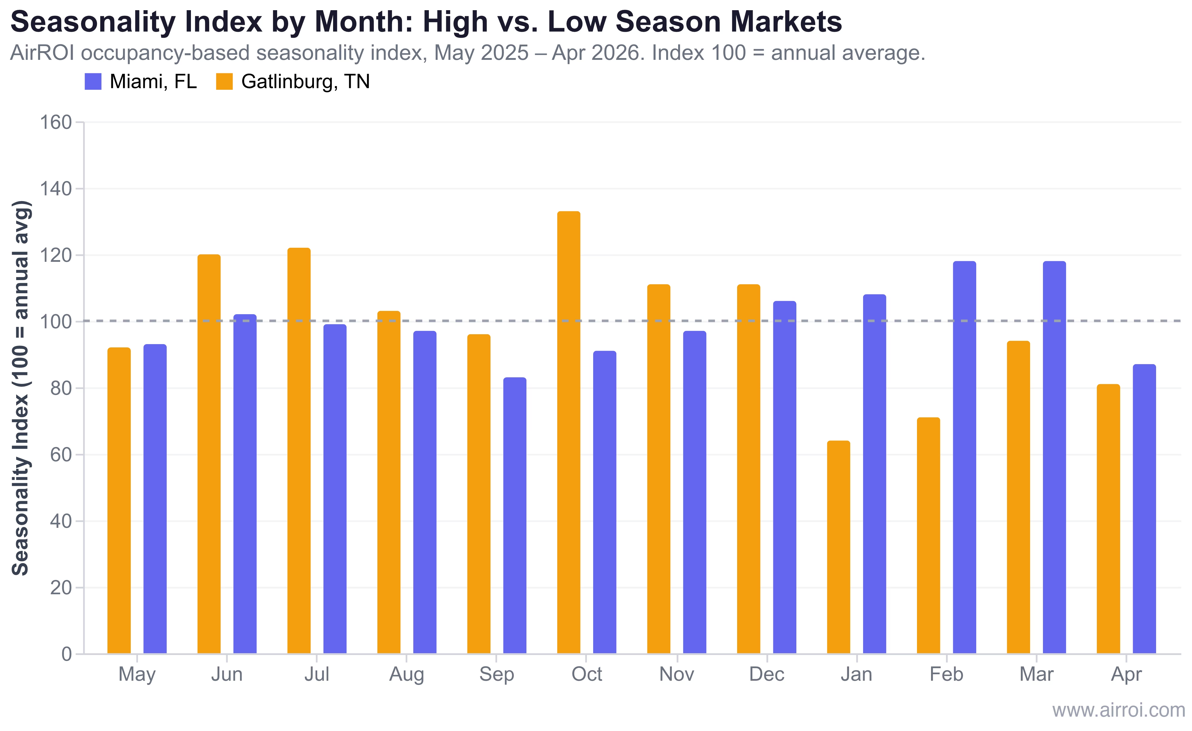
In AirROI's analysis of 13,717 active listings across Miami, FL and Gatlinburg, TN, the two markets illustrate opposite seasonal structures:
- Miami, FL (9,718 listings) — winter-peak market with a 35-point index spread (83 in Sep → 118 in Feb/Mar). Demand is relatively stable year-round, driven by year-round tourism and conference travel.
- Gatlinburg, TN (3,999 listings) — dual-peak mountain market with a 69-point spread (64 in Jan → 133 in Oct). The October foliage peak is the dominant revenue event, while January and February represent a genuine deep off-season.
A Gatlinburg host who prices January the same as October leaves over 50% of peak-month demand on the table — the index spread between those two months is wider than many markets' entire annual range.
The contrast matters most for investors: Gatlinburg's higher ADR ($376.50 vs. $291.00 for Miami) co-exists with a more volatile demand curve, which means cash reserves, minimum-stay rules, and rate strategies must account for genuine slow months in a way a Miami property does not require.
Why the Seasonality Index Matters for STR Operators
Booking pace context. A 40% occupancy rate for July measured in March is strong for some markets and alarming for others. The index tells you what your market's July historically looks like relative to the annual baseline — without it, mid-year booking pace is uninterpretable.
Operations planning. The lowest-index months are the right time for renovations, deep cleans, and professional photography — work that would displace revenue during peak months.
Seasonality Profiles by Market Type
| Market Type | Typical Index Range | Dominant Peak | Off-Peak Driver |
|---|---|---|---|
| Winter-peak beach | 75–120 | Dec–Mar (warmth migration) | Sep–Oct (hurricane season) |
| Summer beach | 55–155 | Jun–Aug | Nov–Feb |
| Mountain/cabin | 60–135 | Jul–Aug + Oct foliage | Jan–Feb post-holiday |
| Ski resort | 55–150 | Dec–Mar snow season | Apr–May, Oct–Nov shoulder |
| Urban business | 85–115 | Weekdays year-round | Holiday weekends |
| Event-driven | 65–180+ | Around major events | Between-event gaps |
How to Build and Apply Your Market's Seasonality Index
- Gather 12–24 months of data — pull monthly occupancy from your STR investment analysis tools or market dashboard. Two years of data smooths out outlier events (a festival cancellation, a major storm) that would otherwise distort a single-year index.
- Compute the annual average — sum all monthly figures and divide by 12.
- Calculate each month's index — divide each month's value by the annual average and multiply by 100.
- Set rate tiers — create at least 4 pricing tiers (peak, shoulder-high, shoulder-low, off-peak) mapped to index bands. A practical split: index ≥120 = peak tier, 100–119 = high-shoulder, 85–99 = low-shoulder, <85 = off-peak.
- Adjust minimum-night requirements — tighten minimums during high-index months to protect peak weekends from short fills that block longer stays. Loosen them when the index drops below 90 to capture incremental occupancy.
- Overlay supply trends — many markets see seasonal supply increases during peak periods as part-time hosts activate listings. If supply rises faster than the index during your peak, competitive pressure may limit the premium you can charge. Use data-driven dynamic pricing to account for this.
- Reassess annually — regulation changes, new infrastructure (highways, airports), and shifting remote-work patterns all alter a market's seasonality curve. The index you computed three years ago may not reflect today's demand structure.
Frequently Asked Questions
A seasonality index is calculated by dividing each month's performance metric (such as occupancy or revenue) by the annual average, then multiplying by 100. A month with an index of 130 is 30% above average, while an index of 70 is 30% below. This normalizes seasonal patterns for easy comparison across markets of different sizes.
A high-seasonality market has large swings between peak and off-peak periods. AirROI data shows Gatlinburg, TN ranging from an index of 64 in January to 133 in October — a 69-point spread. A low-seasonality market stays relatively flat year-round; Miami's index spans just 35 points (83 in September to 118 in February and March), reflecting its year-round tourism base.
Your nightly rates should mirror your market's seasonality index. During months with an index above 100, price above your annual average ADR. During months below 100, lower rates help maintain occupancy. The magnitude of your adjustments should roughly correspond to the index deviation — a market with an October index of 133 warrants rates roughly 33% above baseline that month.
Yes — and it is one of the most valuable uses. Two markets can have similar annual revenue but very different risk profiles. A market with an index range of 64–133 requires more active management, tighter cash reserves for off-peak months, and more aggressive peak pricing than one with a 83–118 range. The index quantifies that operational complexity before you invest.
Seasonality troughs depend on market type. Mountain and cabin markets like Gatlinburg see their lowest index in January and February (post-holiday winter). Beach markets like Miami hit their trough in September at the end of hurricane season. Urban markets experience their deepest lows around major holiday weekends when business travel stops. Always measure the index for your specific submarket, not a national average.